Translate this page into:
Primer of Epidemiology 3: An overview and observational study designs
2 Public Health Foundation of India, Gurugram, Haryana, India
Corresponding Author:
Poornima Prabhakaran
Centre for Chronic Disease Control, C1/52, 2nd Floor, Safdarjung Development Area, New Delhi 110016
India
poornima.prabhakaran@phfi.org
| How to cite this article: Prabhakaran P, Shivashankar R. Primer of Epidemiology 3: An overview and observational study designs. Natl Med J India 2020;33:291-297 |
Introduction
Study designs help investigators to operationalize a conceptual hypothesis of research. These designs include a specific plan, methods and criteria for selecting individuals to make a valid comparison between groups. Epidemiological study designs are broadly classified as observational and interventional studies [Figure - 1]. Observational studies are further stratified as descriptive and analytical. Descriptive studies describe just the observation while analytical studies make comparisons between groups.
![[Figure - 1]](#fig_NatlMedJIndia_2020_33_5_291_317472_f1.jpg)
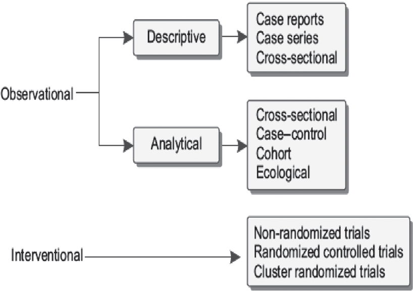 |
| Figure 1: Types of study designs |
Observational Studies
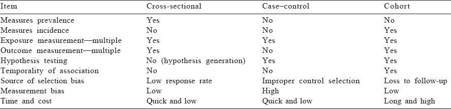
These are epidemiological studies in which the researcher does not intervene or change any of the variables but simply observes and records them. Observational research is a part of epidemiology and usually precedes experimental designs. In many instances, observational research is the only method to draw epidemio-logical inferences as experiments are not possible due to ethical or logistic reasons. [Table - 1] describes various types of observational studies that are discussed in this article.
![[Table - 1]](#tbl_NatlMedJIndia_2020_33_5_291_317472_t7.jpg)
Cross-Sectional Studies
PIMA Indian study
The PIMA Indians, also known as Gila River people, are a group of Native Americans who comprise one of the earliest pre-Columbian migration to the Americas and live in an area what is now central and southern Arizona in the USA. In the 1960s, a pilot survey investigating the seemingly high prevalence of rheumatoid arthritis unravelled a high prevalence of glycosuria and prompted the National Institutes of Health to conduct a formal survey of diabetes in the population. The results of this study published in The Lancet by Bennett et al.[1] documented a shockingly high prevalence of adult-onset diabetes (what is now termed as type 2 diabetes). Although subsequently structured as a longitudinal study, it began as a cross-sectional survey of the residents aged 5 years and older living in the Gila River reservation of Arizona. Diabetes was defined by the 75-g oral glucose tolerance test. Each resident of the study area who was at least 5-years-old was invited for an examination that included medical history, physical examination, oral glucose tolerance test and measurements of height and weight, serum lipids, serum insulin and urinary proteins. A total of 2917 Pima Indians participated in this study. The 2-hour post-load glucose level of >160 mg/100 ml was the cut-off determined for diagnosis of diabetes. The prevalence of diabetes mellitus was 42% among those aged 25 years and older, and 50% among those aged 35 years and older. These findings documented that the Pima Indians had the highest prevalence of diabetes mellitus worldwide at that time. This initial result and subsequent longitudinal follow-up led to the mechanistic understanding of diabetes including the role of insulin resistance (Narayan KMV, personal communication, 2018).[1]
Prevalence of coronary artery disease in Indian migrants
Another study of prevalence of atherosclerosis that led to the enquiry of high propensity of coronary artery disease among Indians compared with that among Chinese and Malays in Singapore was reported by Danaraj et al.[2] Across all age groups, the age-specific mortality due to coronary artery disease was high among Indian males compared with that among Chinese males. This was the first report indicating a high prevalence of coronary artery disease among Indians, which led several other cross-sectional comparisons of Indian migrants with other populations across different parts of the world.[2]
Cross-sectional studies are observational studies that measure an array of risk factors and disease end-points at one point in time [Figure - 2]. They are the primary study design used to describe the characteristics (e.g. sex, age and occupation), risk factor distribution and disease profile of a given target population. The target population for a cross-sectional study is often defined by a particular geographical or institutional setting, such as one or many nations, communities, hospitals and schools.
![[Figure - 2]](#fig_NatlMedJIndia_2020_33_5_291_317472_f2.jpg)
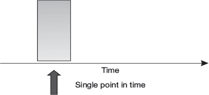 |
| Figure 2: Cross-sectional study |
Cross-sectional studies are highly useful in measuring burden of diseases/risk factors for prioritizing interventions/policies at a hospital/health system/population level. The National Family Health Survey (NFHS) of India is a prominent example of a cross-sectional survey.[3] It uses multistage cluster random sampling to recruit a nationally representative sample of the population. The study reports the current health and nutrition status of residents including the prevalence of historically important health conditions such as underweight and stunting in children. The latest round of this survey (NFHS-4; 2014–2015) also included measures of chronic diseases such as blood pressure (BP) and capillary glucose measurements. These surveys provide evidence to policy-makers about national health status and also provide data for evaluating the performance of many national programmes.[3]
Cross-sectional surveys are often repeated at regular intervals (e.g. the National Health and Nutrition Examination Survey in the United States and NFHS) or arbitrary intervals to provide data on changes in population characteristics and disease profiles over time. These comparisons are valid only when the same sampling methodology is used to identify and recruit participants for the survey at each time-point in question. Such repeated cross-sectional studies measure trends in diseases and risk factors and aid in the revision of health policies. In the National Capital Region of Delhi (NCR Delhi), a cross-sectional survey was conducted during 1991–94 to measure the prevalence of cardiovascular diseases and their risk factors (body mass index, BP, blood glucose and lipids). The survey was repeated after almost 20 years during 2010–12 using the same methodology in a new sample. The comparison of the results of both surveys showed higher levels of cardiovascular risk factors in the latest survey compared with the previous one.[4]
An advantage of cross-sectional studies is that they do not require follow-up of participants and therefore can provide data in a more rapid time-frame than longitudinal studies. Smaller cross-sectional studies with limited biological samples can also be conducted with relatively minimal resources. Furthermore, cross-sectional studies often provide rich data for establishing putative associations between risk factors and diseases in a large population, and therefore, they are highly useful in generation of hypothesis, which can be tested in more rigorous designs later. A limitation of cross-sectional studies is that they cannot confirm the causal relationship between a putative risk factor and a disease because the temporal ordering (direction of association) between an exposure and an outcome cannot be determined.
Relatedly, cross-sectional studies cannot provide data on incidence of new disease because participants are observed only once in time. Cross-sectional studies are suitable for measuring the prevalence of diseases that are of a longer duration and occurring at a high frequency (e.g. hypertension or carotid intima thickness) or degenerative disorders with a clear point of onset (e.g. cardiac failure). They are not suitable for measuring highly fatal or short duration of diseases (Ebola infection or paroxysmal atrial fibrillation). As a corollary to this point, cross-sectional surveys may be affected by survival bias. For example, a cross-sectional study of prevalence of ischaemic heart disease in a low- and middle-income country may find a low prevalence of myocardial infarction (MI). The low prevalence in the community may not be because there is low incidence but due to high case fatality of MI, which is missed in a cross-sectional survey.
Case–Control Studies
The INTERHEART study is a landmark global case–control study that evaluated the effect of behavioural and psychosocial risk factors on coronary heart disease (CHD) with participants from varying ethnic and geographical regions.[5] Before this study, the widely held view was that genetic factors played a large role in the causation of CHD, particularly among certain ethnicities such as South Asians. The study was an international case–control study conducted in 52 countries and enrolled 15 152 cases and 14 820 controls from 262 centres. Patients who reported the symptoms of acute MI and electrocardiogram indications of acute MI were recruited as cases, whereas those with no previous history of heart disease or chest pain were recruited as controls. Standard questionnaires were administered to collect information on sociodemographics, behavioural risk factors and psychosocial factors, and physical examinations were done to record the anthropometric measurements and BP.
Blood samples were collected for total cholesterol, high-density lipoprotein and Apolipoproteins B and A1. Odds ratios and population attributable risks (PARs) were calculated using statistical software. The study concluded that nine major risk factors—abnormal lipids, smoking, hypertension, diabetes, abdominal obesity, psychosocial stress, decreased consumption of fruits and vegetables, moderate consumption of alcohol and physical inactivity—were associated with acute MI among both sexes and in all ages worldwide and accounted for 90% of PAR in males and 94% in females. The study results suggested that prevention approaches for acute MI can be similar throughout the globe, and modifications in these risk factors have the potential to reduce patients with acute MI.[5]
Case–control studies are observational studies in which we attempt to identify the cause(s) of a particular disease. In contrast to cross-sectional studies that tend to be largely for data description, case–control studies are intended to identify associations. In this study design, participants are selected based on the presence or absence of disease. Cases are sampled to have the disease of interest, and controls are sampled to be negative for the disease of interest. Both cases and controls are assessed for exposure status, and the relationship between exposure and disease status is quantified through the odds ratio. Case–control studies are particularly useful for studying rare diseases for which we would otherwise need an extremely large random sample to obtain a sufficient number of diseased individuals for study. Other advantages of case–control studies are that they are quick and relatively inexpensive to conduct. The major disadvantages are that case–control studies are prone to both selection and information bias. Selection bias occurs specifically in the choice of controls (see the subsequent text). Information bias (recall bias and interviewer bias) occurs since the information on exposure is collected after the outcome has occurred. Another disadvantage is that the temporal ordering of the exposure relative to the outcome cannot be established in this design.
A classical case–control study is considered retrospective because the starting point for sampling is the presence or absence of disease (for cases and controls, respectively) and we then retrospectively obtain exposure status (e.g. risk factors) after cases and controls are sampled.
[Figure - 3] describes the case–control design. The design dates back to the 1920s when the first case–control study was conducted to measure association between smoking and squamous cell carcinoma.[6] Case–control designs became more prominent in the 1950s when a series of such studies reported the association between smoking and lung cancer, including the classical study by British scientists Sir Richard Doll and Sir Austin Bradford Hill.[6] Since then, the design has further evolved with the advent of refined approaches to sampling and newer statistical methods for its analysis.
![[Figure - 3]](#fig_NatlMedJIndia_2020_33_5_291_317472_f3.jpg)
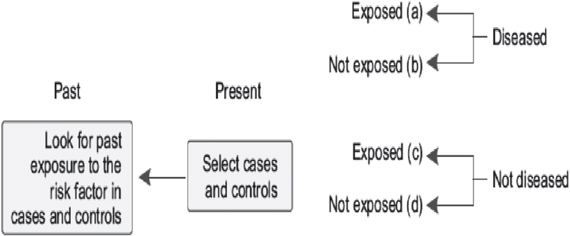 |
| Figure 3: Design of case–control studies |
Features of case–control studies
Case–control studies are highly prone to selection biases. Therefore, careful planning in selection of cases and controls and measurement of exposures is needed to obtain meaningful results from this design. There are five main criteria for conducting a well-designed case–control study:
- Both cases and controls must come from the same base population.
- The sample of controls must be independent of exposure and truly represent the non-diseased in the base population that gave rise to the cases.
- Disease must be convincingly ruled out in controls, and disease must be relatively rare (usually affects <10% of population).
- Exposure determination is done in the same way in cases as well as in controls.
- Sampling should be done in a manner that ensures that had ‘control’ been a ‘case’, it would have been sampled.
Selection of cases
A well-constructed, unambiguous definition of ‘the case’ is the key to the selection of cases. The definition should include age, gender, type and severity of cases and the criteria for selection (clinical, laboratory, histological and/or radiological). It is critical to ensure that cases should have a reasonable probability of having the exposure.
In the INTERHEART study, all the patients admitted in the coronary care units were screened within 24 hours for eligibility to be a case.[5] The study clearly defined a case as a patient of any age and gender having clinical symptoms and electrocardiogram showing diagnostic changes of MI such as new pathological Q waves or 1-mm ST elevation in any two or more contiguous limb leads or a new left bundle branch block or new persistent ST-T wave changes suggestive of a non-Q-wave MI or raised concentrations of troponin. Criteria for subsequent confirmation included a substantially raised concentration of enzymes (>2 times normal) or evolution of electrocardiographic changes. Patients with cardiogenic shock or a chronic medical illness (e.g. liver disease, untreated hyperthyroidism or hypothyroidism, renal disease or malignant disease or who were pregnant) were excluded because these conditions might change lifestyle or alter the risk factors for acute MI.
Incident versus prevalent cases
It is preferable to consider incident (newly developed) cases for case–control studies as was done in the INTERHEART study.[5] There may be a risk of potential biases if prevalent (existing) cases are recruited. Imagine that you are doing a case–control study to assess the relationship between sodium intake (from 24-hour urinary excretion) and hypertension. Should we recruit incident or prevalent patients with hypertension? Patients with previously existing and diagnosed hypertension may have modified their salt intake. If we recruit prevalent cases, the results will show a spurious negative relationship between sodium intake and hypertension, which is not accurate. Therefore, patients newly diagnosed with hypertension should be recruited for this study. The same principle applies to the study of most behavioural risk factors associated with any chronic condition. In contrast to this scenario, prevalent cases may be appropriate when the exposure of interest is a fixed attribute that certainly predates the disease (e.g. genetic factors and birth weight).
There are additional reasons to recruit incident cases. Recall errors of exposure history and symptoms are lower in incident cases. Furthermore, diagnostic criteria for the outcome could have changed over time. This may lead to a heterogeneous mix in cases if the prevalent cases are recruited. Therefore, it is advisable to recruit incident or new cases for case–control studies.
Selection of controls
Selection of controls is the most crucial part of case–control studies. Ideally, controls should have the same probability of selection as cases in the study, that is, a control should be similar to the case minus the disease of interest. Therefore, controls should be recruited from the same community from which the cases were recruited. The most common dilemma in case–control studies is whether to recruit a control from hospitals or from the community. There are pros and cons of both types of controls.
Hospital-based controls
Most studies recruit hospital controls as that is easier to accomplish. Other advantages are that participants are usually motivated and cooperate with investigators, and differential recall of exposure between cases and control is minimal (and therefore reduces recall bias).
Nonetheless, there are two major disadvantages. First, an underestimation of the exposure effect may be obtained if controls are admitted to the hospital for diseases that are aetiologically similar to the case disease. Let us take an example of a case–control study that aims to assess the association between tobacco chewing and MI. Can patients from an oral health clinic be recruited as controls? No, because patients in the oral health clinic have a higher probability of chewing tobacco compared with the general population. Patients from other clinics such as ophthalmology will provide controls that are more representative of the general population in terms of chewing tobacco.
Another common cause for bias occurs when both a putative risk factor and disease play a role in motivating people to go to the hospital. For example, we want to study the relationship between diabetes (putative risk factor) and MI (disease outcome). If controls are recruited from hospitals, we will overestimate the relationship because both people with diabetes and MI are more likely to visit a clinic and therefore are over-represented in our sample as compared with the population. This phenomenon is known as Berksonian bias.
Second, sometimes, hospital controls may not represent the base population that gave rise to case patients, which leads to selection bias. In the same example of tobacco chewing and MI, it is possible that the hospital caters to MI cases of a local urban community (as MI is an emergency condition) but patients for oral health clinics may come from a larger geographical region that also includes rural communities. In such cases, it is recommended to use neighbourhood or community controls.
Community-based controls
Unrelated visitors or neighbours of the index case can contribute to community-based controls. Use of community-based controls reduces selection bias that may arise from hospital controls and makes the results of the study more generalizable. However, there are some disadvantages. Logistically, recruiting these controls is time-consuming and suffers from low response rate, thereby increasing the expenses. The study is prone to recall bias.
To overcome the specific disadvantages of hospital- and community-based controls, it is ideal to recruit two sets of controls—one hospital and one neighbourhood if adequate resources are available.
In the INTERHEART study, both community- and hospital-based controls (those with no history of MI) were recruited.[5] The first control was a community-based control. This was either a visitor or relative of a patient from a non-cardiac ward or an unrelated (not first-degree relative) visitor of a cardiac patient. For the hospital-based controls, the study preferably recruited patients who were more likely to represent the general population such as patients who came in for a refraction test, cataract surgery, physical check-up, routine Papanicolaou smear, routine breast examination, elective minor surgery for conditions that are not obviously related to CHD or its risk factors or elective orthopaedic surgery. However, to improve recruitments, the study also accepted controls if they had attended hospital for outpatient fractures, arthritic complaints, plastic surgery, haemorrhoids, hernias, hydrocoeles, routine colon cancer screening, endoscopy or minor skin disorders.
More than one control per case
When the cases are rare, increasing the number of controls (up to four times) increases the power of the study. This also provides an opportunity to have more than one type of control, for instance, one set of controls from hospitals and another from the neighbourhood.
Matching is a method used in case–control studies to reduce confounding. Controls are matched with cases for common confounders such as age and sex. Matching can be either individual matching (every control is matched with a case) or frequency matching (ensuring equal number of cases and controls in small segments of matching criteria, e.g. 5-year age groups). Number of factors that can be matched should be minimum to avoid overmatching. In the INTERHEART study, controls were individually matched to cases for sex and age (±5 years).[5] The classic and individually matched analyses of case–control studies are shown in [Figure - 4].
![[Figure - 4]](#fig_NatlMedJIndia_2020_33_5_291_317472_f4.jpg)
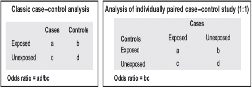 |
| Figure 4: Analysis of case–control studies |
Despite the possibility for selection and information bias, there are major case–control studies across the world that have contributed to cardiovascular epidemiology. The INTERHEART study was one of the major breakthrough studies in cardiology.[5] This study established that nine classic risk factors (smoking, low apolipoprotein A/apolipoprotein B ratio, high BP, diabetes, abdominal obesity, low fruit and vegetable consumption, lack of exercise, alcohol and psychosocial factors) were responsible for 90% of cardiovascular events irrespective of region, ethnicity and gender. The results of this study are cited to this day.
Cohort Studies
Cardiovascular morbidity and mortality were steadily increasing in the USA in the early 1900s. Little was known about the causes or risk factors for these trends. In 1948, a little over 5000 individuals, males and females, 30–62 years of age, residing in the town of Framingham, Massachusetts, were recruited into an ambitious joint project by the National Heart Lung and Blood Institute and Boston University. Baseline examinations and careful follow-up over the following years led to the recognition of common patterns of development of cardiovascular disease, analyses of these pathways and identification of the classical cardiovascular risk factors—high BP, smoking, overweight/ obesity, diabetes, high cholesterol, poor diet and physical inactivity apart from age, gender and psychosocial factors. This classical epidemiological research—the Framingham Heart study[7]—captures the essence of the cohort study design, also known as the longitudinal study design or prospective study design because of the prospective nature of follow-up of the participants. Cohort studies are also called incidence studies as they allow the study of occurrence of new disease or risk factors with sufficient follow-up time.[7]
PIMA study revisited
In the section ‘Cross-sectional studies’, we described a large study of Pima Indians in the Americas. The initial studies on prevalence inspired a longitudinal cohort study in which Pimas aged 5 years and over were followed over a 10-year interval with periodic examinations. A total of 3733 Pima Indians were followed over a 10-year period. Using a 2-hour post-load glucose level of >200 mg/100 ml as the cut-off determined for diagnosis of diabetes, the prevalence of diabetes mellitus was 21%, and the incidence of diabetes was 26.5/1000 person-years. These findings documented that the Pima Indians had the highest prevalence and incidence of diabetes mellitus worldwide at that time.[8]
Description
Cohort studies, classically, do a follow-up on a group of individuals for the development of new cases of a disease under study. Typically, individuals are free of disease or its risk factor(s) at the start of the study. Over time, the individual(s) may or may not develop the risk factor or outcome in question. Cohort studies thus help us quantify ‘risks’ for disease and ‘relative risk’ for disease associated with a particular exposure. A comparison of those who develop the outcome with those who do not helps us understand the potential aetiological pathways to disease occurrence, with respect to their exposure status. [Figure - 5] provides the schema for a cohort study.
![[Figure - 5]](#fig_NatlMedJIndia_2020_33_5_291_317472_f5.jpg)
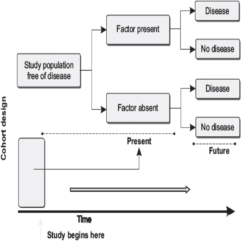 |
| Figure 5: Classical structure for a cohort study design |
Characteristics of a cohort study
A cohort study begins with the recruitment of a specified group of individuals from a designated target population, which may be restricted to a particular area or setting. The process of recruitment, including eligibility criteria, locations and time-frame, is specified at the outset of the study. At the first study visit, termed the baseline visit, information is collected on a number of variables. These variables include data on personal, household and demographic information, education, lifestyle factors such as smoking and alcohol, diet, physical activity and any other information that is relevant to the primary disease end-point. The selected group of individuals, which then becomes the study cohort, is followed up over time. The frequency of follow-up is predetermined, and subsequent visits may include an assessment of the complete cohort or only a subgroup of individuals. The information collected over time is eventually analysed after sufficient measurable risk factors or disease end-points have accumulated. This can vary with the study outcome. Where the development of outcomes/disease end-point may take a long period, researchers may decide to analyse for intermediate end-points. An example is the study of cardiovascular risk factors such as high BP or impaired fasting glucose before the occurrence of hard end-points or outcomes such as MI or death.
Advantages of cohort studies
Cohort studies facilitate description of diseases in populations as well as analysis of causes of disease. They allow us to describe the incidence of disease, study the natural progression of a disease, measure changes in the status of risk factors over time, assess the temporal sequence of events between exposure and outcome and study the rare exposures. They can also often be repurposed or reanalysed to examine multiple outcomes.
Limitations of cohort studies
Cohort studies involve the investment of time, money and resources. There is an inherent disadvantage of loss of individuals during follow-up (attrition), and this can lead to interpretation bias. Selection bias can also occur at baseline. Changes in the status of risk factors can occur over time. For example, a smoker at baseline may give up smoking at a later point during follow-up—this should be actively monitored during follow-up examinations. There may be an exposure misclassification owing to lack of sufficient reliable data at baseline and this can affect results of the study. Outcome bias is also possible if the assessment of outcome is influenced by knowledge of the exposure status. While not specific limitations of cohort studies, confounding, information bias and lack of precision may also threaten a valid inference.
Types of cohort studies
Prospective. Classical cohort studies follow individuals prospectively over time to collect information. These are also called concurrence studies because of the concurrent nature of follow-up. This involves regular follow-up of a large set of individuals, maintenance of trained staff over prolonged periods of time to conduct the examinations in a standardized manner and then wait for the occurrence of study end-points—often difficult when the disease under question is rare.
Retrospective (historical). As the name suggests, this design allows investigators to overcome the constraints of time and some resources using data that already exist. For example, a group of individuals whose medical records are available can become the cohort population. Using these existing medical records, patients are classified according to exposure and disease status and the interval between the first report of the exposure and the development of disease. The relationship between the exposure and disease can be quantified on this retrospectively constructed cohort study. This saves time and resources for setting up the study and following up in time for data collection.
Another example is the use of health records in an industrial population. If a specific occupational disease is being studied, it is most feasible to select an appropriate industrial site, assemble a cohort of study participants and seek previous health records to determine their exposure status. A group of individuals not exposed to the potential exposure, within the same factory, could serve as a comparison group. Consider exposure to lead and its relationship with hypertension among workers in a printing press. Employees on the administrative or clerical side or those who bind books on the site can serve as controls while workers within the printing units, with direct occupational exposure to lead, form the study participants. While a retrospective design helps to save time, there are inherent disadvantages too because the source of data may not be complete or reliable for research purposes. Health records, for instance, may not be collected with a research focus and detailed questioning may not have been done to capture data that may be required to meaningfully interpret results.
Combined retrospective and prospective cohort. A combination of the above-mentioned two designs involves the use of medical records or other health data collected previously (retrospective), assessing the cohort members in the current time and then also following them forward in a prospective manner to assess the development of risk factors or outcomes. This benefits from not only easy cost-effective assembling of the study group but also assessing the incidence of disease in real time.
Birth cohorts
An interesting and widely used study design is the birth cohort. As the name suggests, this usually involves a cohort of individuals assembled at birth. Women may be recruited before or during pregnancy with a lot of useful information and measurements collected at baseline. Once births occur, usually defined as a specific period of time, the babies are also recruited and constitute the birth cohort. The entire cohort is followed up in time, sometimes over years and decades, with multiple rounds of data collection on the whole or part of the cohort, and various outcomes studied. Birth cohorts are an extremely useful resource and have been used worldwide to provide important insights into many mechanistic pathways of disease, especially with an intergenerational focus. Such studies use maternal nutritional, sociodemographical, environmental, medical and other information to study the role of early life influences on later-life risk of disease in the offspring of the next and subsequent generations.
The New Delhi Birth Cohort was established in 1969, including all births within a defined radius in South Delhi, that occurred between 1969 and 1972, a total of 8181 births. The cohort has been followed up for four decades with a rich repository of research on growth, metabolism and cardiometabolic disease. A drawback in such studies is the huge cost, participant exhaustion or migration and resulting loss to follow-up over time, leading to attrition, which may affect results. The New Delhi Cohort, for example, has a little over 2000 individuals under follow-up now, but also included parents, spouses and the children in the next generation in several studies.[9] Similar cohorts elsewhere include the Avon Longitudinal Study of Parents and Children in Bristol, United Kingdom,[10] the Generation R cohort in Rotterdam[11] and a Guatemalan birth cohort (INCAP study)[12] in South America, among several others, which have all provided tremendous insights into disease patterns, incidence and mechanistics.
Case–cohorts and nested case–control
This is a modified design where for some outcomes/exposures, only a subgroup of the original cohort is followed. The subgroup typically includes all incident cases of the disease who are observed during follow-up and some proportion of cohort at baseline (case–cohort) or controls who never develop disease (nested case–control). These sophisticated designs capitalize on the rich data infrastructure provided by the parent cohort study but reduce further cost of studying of more outcomes.
Analysis and interpretation of a cohort study
Cohort studies use information on the presence or absence of exposure to assess the incidence of disease over time. Individuals who develop the outcome and those who do not are compared with respect to their exposure status to calculate the incidence of disease in the two groups [Figure - 6]. This comparison allows inference on the possible association between the studied exposure(s) and the outcome. Risk and rates (including disease incidence) and measures of association based on the risk and rate can usefully be computed from cohort data. For further details refer to Primer of Epidemiology 1: ‘Measures of occurrence’ and ‘Studying associations as a path to understanding causation’.[13]
![[Figure - 6]](#fig_NatlMedJIndia_2020_33_5_291_317472_f6.jpg)
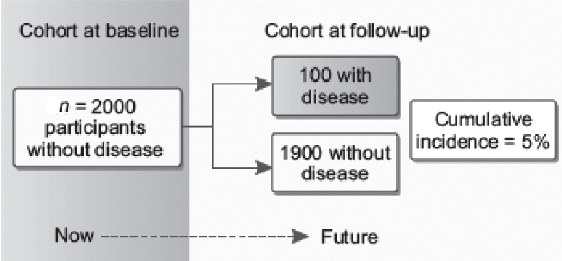 |
| Figure 6: Analysis of cohort studies. The figure shows how participants without disease are enrolled in a cohort at baseline and are later followed up over time to observe the accumulation of disease. Among the 2000 participants at baseline, 5% developed disease; therefore, the cumulative incidence is 5% |
Cohort studies are therefore a useful observational study design when sufficient time and resources are available to the researchers, allowing the study of rare exposures and where disease of interest is common. Special designs such as occupational cohorts and birth cohorts are also useful.
Acknowledgements
We are grateful to Professor Prabhakaran Dorairaj, Vice-President, Research and Policy, Public Health Foundation of India; Executive Director, Centre for Chronic Disease Control for conception of the idea of this series on Primer of Epidemiology and for his careful guidance and editing of the original publication of the Epidemiology section in Tandon’s Text Book of Cardiology. We are also grateful for diligent assistance with editing and referencing by Ms Sanjana Bhaskar, Senior Research Assistant at the Centre for Environmental Health at the Public Health Foundation of India.
Conflicts of interest. None declared
| 1. | Bennett PH, Burch TA, Miller M. Diabetes mellitus in American (Pima) Indians. Lancet 1971;2:125–8. [Google Scholar] |
| 2. | Danaraj TJ, Acker MS, Danaraj W, Wong HO, Tan BY. Ethnic group differences in coronary heart disease in Singapore: An analysis of necropsy records. Am Heart J 1959;58:516–26. [Google Scholar] |
| 3. | National Family Health Survey, India. Available at http://rchiips.org/nfhs/ (accessed on 16 Feb 2018). [Google Scholar] |
| 4. | Roy A, Praveen PA, Amarchand R, Ramakrishnan L, Gupta R, Kondal D, et al. Changes in hypertension prevalence, awareness, treatment and control rates over 20 years in national capital region of India: Results from a repeat cross-sectional study. BMJ Open 2017;7:e015639. [Google Scholar] |
| 5. | Yusuf S, Hawken S, Ounpuu S, Dans T, Avezum A, Lanas F, et al. Effect of potentially modifiable risk factors associated with myocardial infarction in 52 countries (the INTERHEART study): Case–control study. Lancet 2004;364:937–52. [Google Scholar] |
| 6. | Doll R, Hill AB. Smoking and carcinoma of the lung; preliminary report. Br Med J 1950;2:739–48. [Google Scholar] |
| 7. | Dawber TR, Moore FE, Mann GV. Coronary heart disease in the Framingham study. Am J Public Health Nations Health 1957;47:4–24. [Google Scholar] |
| 8. | Knowler WC, Bennett PH, Hamman RF, Miller M. Diabetes incidence and prevalence in Pima Indians: A 19-fold greater incidence than in Rochester, Minnesota. Am J Epidemiol 1978;108:497–505. [Google Scholar] |
| 9. | Bhargava SK, Sachdev HS, Fall CH, Osmond C, Lakshmy R, Barker DJ, et al. Relation of serial changes in childhood body-mass index to impaired glucose tolerance in young adulthood. N Engl J Med 2004;350:865–75. [Google Scholar] |
| 10. | Fraser A, Macdonald-Wallis C, Tilling K, Boyd A, Golding J, Davey Smith G, et al. Cohort profile: The Avon longitudinal study of parents and children: ALSPAC mothers cohort. Int J Epidemiol 2013;42:97–110. [Google Scholar] |
| 11. | Jaddoe VW, Mackenbach JP, Moll HA, Steegers EA, Tiemeier H, Verhulst FC, et al. The generation R study: Design and cohort profile. Eur J Epidemiol 2006; 21:475–84. [Google Scholar] |
| 12. | Stein AD, Melgar P, Hoddinott J, Martorell R. Cohort profile: The Institute of Nutrition of Central America and Panama (INCAP) nutrition trial cohort study. Int J Epidemiol 2008;37:716–20. [Google Scholar] |
| 13. | Patel SA, Prabhakaran P. Primer on Epidemiology 1: Building blocks of epidemiological enquiry. Natl Med J India 2020;33:45–50. [Google Scholar] |
Fulltext Views
2,275
PDF downloads
362


