Translate this page into:
Primer on Epidemiology 2: The elements of study validity and key issues in interpretation
2 Centre for Chronic Disease Control, New Delhi, India
Corresponding Author:
Shivani Anil Patel
Global Health and Epidemiology, Emory University, 1518 Clifton Road NE, CNR 7037, Atlanta, Georgia 30322
USA
s.a.patel@emory.edu
| How to cite this article: Patel SA, Shivashankar R. Primer on Epidemiology 2: The elements of study validity and key issues in interpretation. Natl Med J India 2020;33:160-165 |
Introduction
In Primer on Epidemiology 1, we outlined the history of epidemiology, the concepts behind rates and risks and how it is applied to populations and individuals. Measurement is an important component of epidemiology. It includes questionnaires, physical measurements as well as laboratory measurements. The conclusions we draw from these measurements determine how accurate the results are and the interpretation of those results. Further, the purpose of our research is to link an exposure (e.g. smoking) to an outcome (e.g. myocardial infarction [MI] or cancer). However, many of the outcomes are multifactorial; they may also be influenced by factors such as confounders and effect modifiers. Further, several biases creep in while we collect our research data. It is important that we address these at the outset so that our study is well designed and yields credible results. These issues are discussed in this article.
Measurement and Error
Both epidemiological and clinical studies rely on accurate measurements. A study measure is the variable that we actually assess and record for our analysis. As mentioned above, these could be questionnaires, physical measurements and laboratory analysis of biomarkers.
Broadly, two kinds of errors are acknowledged in epide-miological studies: (i) random and (ii) systematic. Random error and systematic error can affect the measurement of exposures, outcomes and other study variables, and also estimation of measures of association. This section focuses on applying the concept of error to the measurement of variables under study.
Random error refers to chance differences between the ‘truth’ and what we measure as investigators. These chance differences do not possess any pattern, i.e. there is no systematic difference between the truth and what we measure. On the other hand, systematic error refers to differences that are predictable and have a pattern (whether or not we recognize the pattern). The classic analogy is the dartboard. Random errors are shown in [Figure - 1]a, and systematic errors are shown in [Figure - 1]b.
![[Figure - 1]](#fig_NatlMedJIndia_2020_33_3_160_314011_f1.jpg)
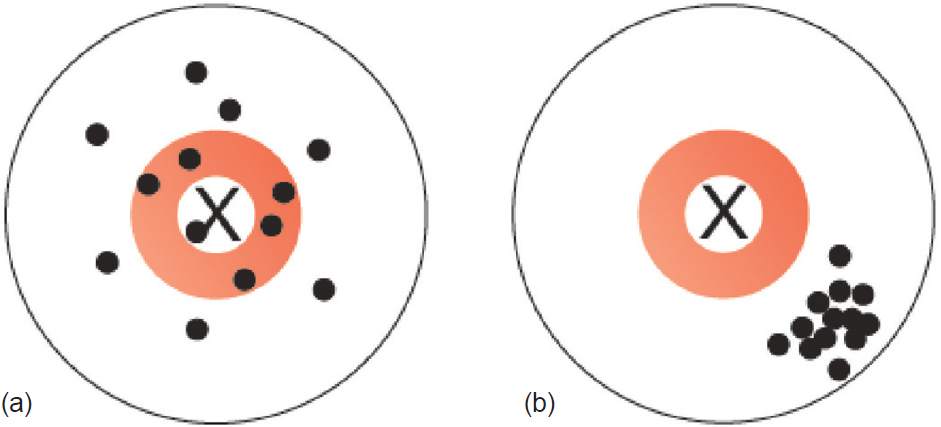 |
| Figure 1: (a) Random error and (b) systematic error |
Coming back to the weighing scale, there may be some random error in the measurement based on the quality of the scale, whether the scale is on an absolute flat surface, and so on, so that on average we capture the true weight of all participants but each participant’s weight may be off by ±0.5 kg. On the other hand, systematic error would occur when, for example, there is a problem with the scale such that it under-weighs all participants. Because the measured weight deviates from the true weight in a consistent and predictable error, we call this scenario systematic error. Random error can be overcome by increasing the sample size, but addressing systematic error would need replacement of the equipment or applying a correction factor estimated using a perfect tool.
Another more complex example is measurement of MI in a sample. There are many ways that MI can be measured operationally in a study. Study participants may be asked to report whether they ever experienced an MI. This ‘self-reported’ measure of MI would be an error-prone measure because there are also silent MIs that go unnoticed; also others may have experienced chest pain but not attended a hospital to get clinically diagnosed. In this way, a person’s true experience of MI may differ from what is recorded in a study using self-reported data only. Alternate ways of measuring MI include review of hospital records, examine electrocardiogram findings and/or cardiac biomarkers that indicate heart muscle cell damage. Each of these approaches has its own set of advantages and disadvantages, such as expected degree of error, cost, invasiveness and feasibility.
Pitfalls Relating to Measurement of Validity and Reliability
Measurement error can lead to problems for both validity and reliability of a study measure. A valid measurement is one that truly measures what it is supposed to measure; for example, if it has a positive measurement, is the true disease status positive? Reliability, on the other hand, is how consistent the measurement tool is; e.g. if we repeat the test, do we get similar values? In [Figure - 2], the X in the centre marks the ‘truth’. [Figure - 2]a shows the results of an ideal measurement tool; it is both close to the truth (valid) and consistent (reliable). [Figure - 2]b shows a measure that is reliable, but not valid; [Figure - 2]c and [Figure - 2]d show results that are not reliable and are therefore of limited use.
![[Figure - 2]](#fig_NatlMedJIndia_2020_33_3_160_314011_f2.jpg)
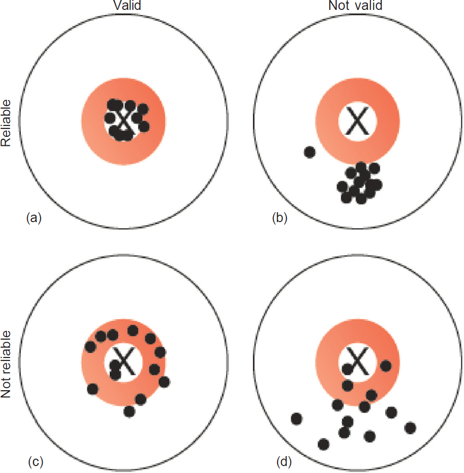 |
| Figure 2: Validity and reliability. The X represents the ‘truth’ and the dots represent our measurement of the truth; (a) measurements that are reliable and valid; (b) measurements that are reliable but not valid; (c) measurements that are not reliable but reasonably valid; (d) measurements that are neither reliable nor valid |
For example, suppose we are collecting the weight of all participants, each participant has a ‘true’ weight in kilograms that we measure with a weighing scale. The question we ask is how reliable are the measurements, i.e. under similar conditions how consistently are we getting same weight? Another metric of measurement is validity. Validity refers to how accurate is the weight measurement by this given scale. The weighing scale may be consistently giving the same weight for participant multiple times and hence reliable. But if the measured weight is consistently 3 kg lower, the weight scale inaccurate and hence has poor validity.
Sensitivity and Specificity
Because much of epidemiology relies on distinguishing between a diseased and a non-diseased state, we often deal with binary variables (also known as dichotomous variables; these are measured as ‘yes’ or ‘no’). Common accuracy measures for binary variables that are used in clinical settings include sensitivity, specificity, positive predictive value (PPV) and negative predictive value (NPV). To calculate these measures, a sense of the ‘truth’––often referred to as a gold standard–– is necessary. [Table - 1] shows a cross-classification between what is measured in a study (on the left-hand column) and the true disease status based on a gold standard test (in the top row). True-positives are individuals who are classified as having disease based on the test measure and truly have disease; false-positives are those who are classified as having disease based on the study measure but truly are disease-free. Similarly, those who are classified as disease-free using the study measure may truly have the disease (a false-negative result) or may be truly disease-free (true-negative). Some of these concepts are explored in detail in other articles of this series.
![[Table - 1]](#tbl_NatlMedJIndia_2020_33_3_160_314011_t5.jpg)
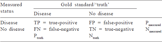
Sensitivity refers to how well the study measure correctly captures disease or the proportion of those with disease who will be correctly classified as having disease: TP/Ptruth. Specificity refers to how well the study measure correctly rules out disease, or the proportion of those without disease who will be correctly classified as having no disease: TP/Ntruth. Sensitivity and specificity must always be balanced in our studies, and it is up to the investigator to prioritize one over the other.
Conversely, a clinician may want to know: What is the chance that her patient has a disease if there is a positive test result? This is referred to as PPV and is computed as TP/Pmeasured. Similarly, NPV is the probability that a patient does not have the disease if there is a negative test result and is computed as TN/Nmeasured.
These metrics are often used for the purposes of determining what cut-off value should be used to classify a disease, how well a test predicts a future condition, understanding how well a cheaper test correlates with a more expensive test or screening which individuals will be targeted for more expensive tests.
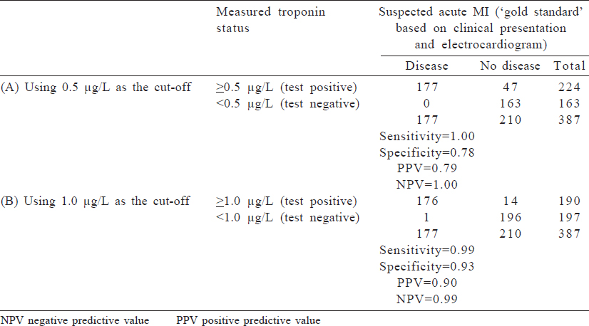
Measurement of sensitivity and specificity is an important concept as diagnostic testing becomes more advanced. An example is a cardiac troponin test to diagnose a suspected MI and to manage acute coronary syndromes. Troponin is a protein that is released in response to damage to cardiac muscle, and because it is relatively specific to cardiac muscle injury, higher levels of serum troponin are considered a diagnostic test to assess an acute MI. The decision of exactly what quantity of serum troponin is considered indicative of an acute MI is a matter of balancing sensitivity (i.e. a level that is low enough to capture cases of acute MI) and specificity (i.e. a level that is high enough to rule out people who do not have an acute MI). We can use previously published data comparing measured troponin-T and clinically disgnosed acute MI to determine the cut-off that meets our needs. A troponin T cut-off of ≥0.5 μg/ L had 1.0 sensitivity and 0.78 specificity, but a cut-off of ≥1.0 μg/ L had a lower sensitivity (0.99) and higher specificity (0.93). Depending on what the clinical system values, the cut-off may be altered. The data from a 1991 study are shown in [Table - 2].[1]
![[Table - 2]](#tbl_NatlMedJIndia_2020_33_3_160_314011_t6.jpg)
Pitfalls Relating to Study Validity
Study validity is described in terms of internal and external validity. Internal validity refers to the scientific robustness of the results of a study and the accuracy of correct results for the study population. For example, if a clinical trial has properly randomized patients, ensured optimal adherence to the intervention and correctly measured the outcome on all patients, the results will likely be internally valid and are deemed trustworthy. Most guidance on research methodology focuses on ensuring that results are internally valid. External validity refers to generalizability, i.e. whether the study results apply to other groups of individuals. Generalizing results across setting presumes that patients are biologically comparable across those settings and that external factors impacting patient pitcomes are also similar. However, generalizing results is fraught with difficulties in practice. For example, most large clinical trials on diabetes were conducted in either the USA or Europe, and the study results may not be applicable to, say, Indians, who may have different levels of key risk factors than previously studied groups. This may be because the biology of diabetes may differ between white populations in the USA (high insulin resistance) and Indians (high beta-cell dysfunction). A new drug that acts by increasing insulin sensitivity if tested and found effective in a study of white adults in the USA cannot be extended without further examination to the Indian population because of differences in prevalent mechanisms of diabetes between the two populations. Apart from biology, there could be other differences across populations that prevent generalizability across settings, including behaviour, compliance, cultural practices and so on, which may influence external validity.
Pitfalls in Internal Validity
There are several threats to study internal validity, or factors that cause the findings of our study to be invalid or untrue reflections of the question of interest. These include lack of precision, information bias, confounding, selection bias and lack of temporal order. The terminology given in the subsequent text is largely applied to measures of association in epidemiology that threaten our ability to test the hypothesis of interest.
Lack of precision
One threat to validity of inference is the lack of statistical precision in estimation. Even when investigators conduct the study perfectly (i.e. there is no systematic error in the data), there is always a possibility of error due to chance, because we are studying only a sample of the full population of interest. For example, if our sample size is small, the estimate we obtain may be unstable and not reflect the true population measure of interest. Statistical precision can be improved through larger sample size.
Bias
Bias most typically refers to a lack of internal validity due to systematic error. It results in deviation from the truth. Bias may arise in many different ways; these are known as threats to validity. The chief threats to validity in epidemiological studies are: Information bias, confounding bias and selection bias. Regardless of the reason, we would say any estimate that systematically deviates from the truth is a biased result. Note that this is different from the common use of the term ‘bias’ in science, which implies false evidence due to partiality of the scientist. Even impartial scientists can produce biased results, and partial scientists can produce unbiased and valid estimates.
Information bias
This refers to bias in a measure of association due to error in the measurement of variables. Both random and systematic error (described earlier) can lead to a biased result. In general, but not always, random error will lead to attenuation of a measure of association, leading to an under-estimation of the true effect. Systematic error may attenuate or enhance the true effect.
Types of systematic error include selective under-reporting of negative behaviour (social desirability bias), selective recall and selective diagnosis. Some methods of measurement are more prone to error than others. For example, an MI ‘diagnosis’ based on a patient’s self-report alone is subject to error because these signs may also reflect other conditions such as chest pain due to oesophageal spasm or reflux. If we use a patient’s medical history as diagnostic evidence, we may also miss a silent MI because the patient would have never sought care if he/she did not experience symptoms. We further divide measurement error into two types: (i) differential and (ii) non-differential. Differential error is error in the measurement that is associated with the exposure; non-differential error is error that is not related to the exposure. Hence, if the same weighing scale is used for all participants in a trial, the error related to the weight measurement should be non-differential because the same tool was used for everyone. On the other hand, if a valid weighing scale was used for all participants of the control arm of a study, but a weighing scale that overestimates weight was used for the intervention arm of a study, we have a case of differential measurement error and we may get a biased association between the treatment and weight status. Recall bias is commonly observed in research, particularly in case–control studies. A patient with acute MI is more likely to under- or over-report an exposure (e.g. physical inactivity or family history) compared with a normal control.
Confounding
Confounding can affect study findings due to the presence of one or more variables that influenced the outcome(s) but may or may not have been accounted for in the study. A confounder in epidemiology is defined as a variable that (i) is related to the exposure; (ii) independently influences the outcome, in the absence of the exposure; and (iii) is not on the causal pathway, i.e. confounder is not a result of the exposure. Referring back to the concept of cause used by epidemiologists, confounding occurs when the apparent association between an exposure and an outcome is not because the exposure causes the effect but because another factor is related to the exposure and outcome and induces a statistical correlation between the exposure and an outcome even when there is no causal association. A positive confounder is a variable that makes the association appear stronger than it actually is, i.e. moves the effect estimate away from the null value. In the presence of positive confounding, the unadjusted estimate is stronger than the adjusted estimate. A negative confounder (masking) is a variable that makes the association appear weaker than it actually is, i.e. one that moves the effect estimate towards the null. In the presence of negative confounding, the unadjusted estimate is closer to null than adjusted estimate.
Example. A researcher wants to study the relationship between coffee consumption and coronary heart disease (CHD). When the researcher creates a 2×2 table of high coffee consumption and presence of CHD, she finds a strong association. The result, however, may be biased because most heavy coffee drinkers are also smokers in our population; therefore, the relationship between smoking and coffee drinking confounds the association between coffee drinking and CHD that is primarily being assessed. The confounder, smoking, is a well-known risk factor independently capable of influencing the outcome of interest (CHD); however, it is not on the causal pathway, i.e. coffee drinking does not cause CHD through cigarette smoking. Cigarette smoking, therefore, satisfies all three prerequisites to qualify as a confounder of the association between coffee consumption and CHD. It is related to the exposure, independently influences CHD and does not lie on the causal pathway. To get an unbiased association, the researcher must account for the relationship between coffee drinking and smoking in the analysis. The most common ways of doing this are conducting separate analysis of the association between coffee consumption and CHD in smokers and nonsmokers (called a stratified analysis) or using software to compute ‘adjusted’ models.
Addressing interpretation pitfalls and accounting for confounders in epidemiological studies. The issue of confounders is central in most epidemiological studies assessing associations between defined exposures and outcomes and must be addressed. Confounding can be dealt with at different stages—study design, analyses and reporting.
- Design stage: At the design stage, we try to select participants so that the confounder distribution is equal in those exposed and unexposed. Matching participants on potential confounding variables (e.g. age) is one approach. We may restrict our study to one level of a confounder to remove the influence of that confounder. For example, if we restrict our study to a specific age group, we would reduce the confounding effect of age on the estimates. Randomization in intervention studies is expressly used as a tool to equalize the distribution of confounders between the intervention and control groups; therefore, potential confounding variables have a minimal impact on the findings from randomized studies. Finally, to enhance confounder control in the analysis stage, a researcher must collect information on all possible confounding factors, based on previous studies or from knowledge of biological plausibility. Exercising judicious choices for data collection during the design stage is central to have sufficient information to conduct a proper analysis
- Analysis stage: There are multiple statistical tools to account for confounding, including stratification, standardization and regression analysis. Each of these tools attempts to eliminate the impact of the confounder in a different way. Stratified analysis involves computing measures of association separately for each level of the confounder (e.g. computing a separate measure of association among smokers and non-smokers), thereby preventing any association between the confounder and outcome to impact results [Figure - 3]. Standardization involves reweighting observations across confounding variables so that the distribution of confounders is more similar across the groups being compared. Multivariable regression models compute a measure of association adjusted for the confounding variable and is the best approach to deal with multiple confounders. Each of these approaches requires the researcher to have collected the appropriate information during the design to incorporate into the analysis. Furthermore, despite comprehensive data collection, always remember that residual confounding can remain because the data we collected do not measure the full impact of confounding variables.
- Reporting stage: We should report all methods used to address confounding in publications. This includes descriptions of confounding variables and presentation of adjusted analyses. In addition, a researcher can communicate hypothesized causal relationships and confounding factors using causal diagrams. [Figure - 4] shows a simple causal diagram depicting the potential relationships among the factors under study; arrows indicate the hypothesized direction of associations. Drawing on our example above, coffee consumption is our exposure of interest (X), smoking is the potential confounder of concern (Z) and CHD is our outcome of interest (Y). [Figure - 4]a shows that coffee causes CHD and that smoking plays no role in this association because there is an arrow directed from coffee to CHD, but there is no arrow connecting smoking with the other variables. [Figure - 4]b shows that coffee consumption causes CHD, but also that smoking is a cause of both coffee consumption and CHD. In this scenario, the observed association between coffee consumption and CHD is partially due to smoking. [Figure - 4]c shows a scenario where coffee consumption does not have any casual effect on CHD. Yet, because smoking is associated with coffee drinking and causes CHD, we would observe a statistical correlation between coffee consumption and CHD if we did not adjust for smoking, despite the lack of a causal effect. If [Figure - 4]c is true, any observed association between coffee consumption and CHD is fully confounded by smoking and should disappear in a stratified analysis (described in more detail later). We must rely on the data to determine which of the diagrams best fits reality and this becomes the knowledge base for clinical guidance.
![[Figure - 3]](#fig_NatlMedJIndia_2020_33_3_160_314011_f3.jpg)
![[Figure - 4]](#fig_NatlMedJIndia_2020_33_3_160_314011_f4.jpg)
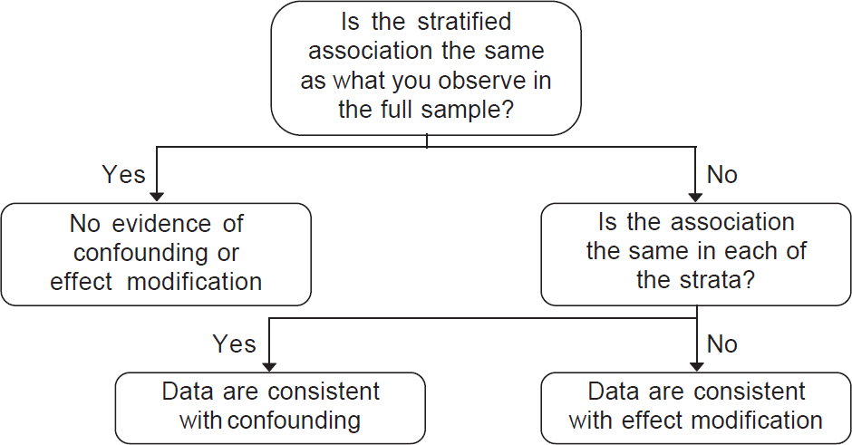 |
| Figure 3: Empirically assessing a confounder versus effect modifier |
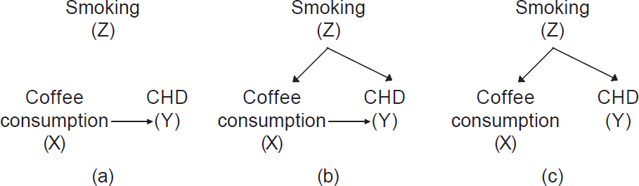 |
| Figure 4: Simple casual diagrams showing potential associations between coffee consumption (exposure) and coronary heart disease (outcome) with and without smoking (Z). (a) A causal association between coffee consumption and coronary heart disease without confounding by smoking; (b) a causal association between coffee consumption and coronary heart disease with confounding by smoking; (c) no causal association between coffee consumption and coronary heart disease but confounding by smoking |
These causal diagrams may also guide the design of our study by suggesting which variables we should collect. They may guide the analysis of our study by helping us think about which variables should be controlled for in the analysis through the methods described earlier.
To summarize, a confounder is a third factor that is associated with the exposure and independently affects the risk of developing the disease. It distorts the estimate of true relationship between the exposure and the disease: It may result in an association being observed when none in fact exists, or no association being observed when a true relationship does exist. It is important to remember that the topic of confounding is vast and investigators take differing approaches to definitions.
Selection Bias
In epidemiology, selection bias refers specifically to when the results are biased because participants were selected using factors that are related to both the exposure and an outcome. Therefore, selection bias is induced through some component of the study or analytical design, and sometimes, aspects of the study that are not in the control of the investigator. Factors leading to selection bias can arise anywhere from the beginning of the study to the analysis stage. For example, at enrolment, self-selection of individuals into the study or the investigator’s choice of where to recruit cases and controls may induce selection bias. A classical example of a selection bias in a case–control study is recruitment of cases (MI) from a corporate hospital and all controls from a nearby slum. Given the huge socioeconomic differences, we may end up with strange incorrect results because the cases and controls are simply not comparable. In longitudinal studies, selective drop-out of sick participants may induce selection bias; similarly, restricting the analysis to individuals who have provided complete data can induce selection bias if providing data was related to the exposure and outcome.
Temporal Order
Finally, and possibly most importantly, internal validity can be threatened through unclear timing of exposure and outcome. A well-designed study would collect exposure data prior to the outcome because the outcome may influence the exposure and lead to spurious results. For example, we would ideally want to measure fruit and vegetable intake prior to the incidence of the first MI because diagnosis of an MI may lead an individual to adopt lifestyle changes such as increased fruit and vegetable intake. If we measured fruit and vegetable intake after the MI, we would get a skewed picture of the true consumption preceding the attack. Another example of the importance of temporal order is when considering two correlated risk factors. For example, consider the relationship between depression and diabetes, two risk factors for cardiovascular disease. Imagine that we observe a positive association between the current depressive symptomatology and measure current HbA1c levels in a cross-sectional survey. We would not be able to discern whether the depressive symptoms preceded the elevated HbA1c levels or the other way round. This is often the justification for conducting prospective studies, in which individuals with existing disease may be excluded in the sample or from the analysis when examining risk factors for developing incident disease.
Effect Modification and Interaction
As you may have noted in clinical practice, not all medications have the same effect in all patients. In fact, some medications are contraindicated for certain groups of people. The phenomenon in which response to a particular intervention or exposure varies by subgroup is termed ‘effect modification’ in epidemiology, because the effect of the intervention or exposure is modified by another factor. An example of effect modification is dual antiplatelet therapy (DAPT) in secondary prevention. While DAPT can increase ultimate survival in post-MI patients, it may indeed reduce survival in CHD patients who have a bleeding peptic ulcer at least in the short term. Thus, the effect of DAPT on survival is expected to vary by bleeding stomach ulcer status.
The term ‘interaction’ is sometimes used synonymously with effect modification. In biological interaction, two treatments may ‘interact’ with one another to produce an effect that is different from what is expected had the treatments been taken in isolation. Potential treatment interaction can be tested in trial settings, although often treatments do not truly interact as hypothesized. One example is the ISIS II Trial, which examined the effects of streptokinase and aspirin alone and in combination on vascular mortality among individuals with suspected acute MI. Survival at year 2 of follow-up among those randomized to streptokinase and aspirin was 4.2% higher than that of the placebo group, while survival among those taking streptokinase alone was 2.6% higher and among those taking aspirin alone was 1.7% relative to respective placebo groups. As the survival benefits of both amounted to the sum of the two treatments (additive effects), the combined treatment did not meet the criteria for interaction. (For a further discussion on effect modification and interaction you could read an article by TJ VanderWeele.[2])
Comparing Confounding to Effect Modification
In confounding, some variable apart from the treatment under study alters the observed relationship between the treatment and an outcome. In effect modification, the effect of the treatment is different over levels of another variable (e.g. age, sex, nationality). While the distinction between confounding and effect modification is also beyond the scope of this article, it is important to be aware that such distinctions exist in the epidemiological literature ([Figure - 3] shows a decision tree when the data are consistent with confounding, effect modification or neither). In confounding, the results in the stratified sample will be the same in all levels of the confounder, but different from those in the full sample. In effect modification, the results will be different in each stratum, and these will differ from those in the full sample.
Hypothesis Testing
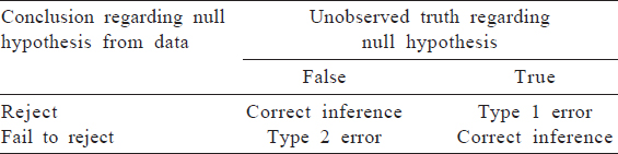
We have discussed errors in measurement and inference. These errors can lead to error in our evaluation of a hypothesis. In hypothesis testing, we attampt to arrive at conclusions regarding our research question based on the data at hand. The possibilities regarding our conclusion in reality and the unobserved truth are shown in [Table - 3]. While Type 1 and Type 2 error in relation to statistical inference will be more fully addressed in the statistical methods, it is useful to think about the validity of our findings in this framework. All the factors that might lead to incorrect conclusions about our hyporgesis are threats to validity.
![[Table - 3]](#tbl_NatlMedJIndia_2020_33_3_160_314011_t7.jpg)
Conflicts of interest. Nil
| 1. | Katus HA, Remppis A, Neumann FJ, Scheffold T, Diederich KW, Vinar G, et al. Diagnostic efficiency of troponin T measurements in acute myocardial infarction. Circulation 1991;83:902–12. [Google Scholar] |
| 2. | VanderWeele TJ. On the distinction between interaction and effect modification. Epidemiology 2009;20:863–71. [Google Scholar] |
Fulltext Views
1,259
PDF downloads
243


